Cracking the Monty Hall problem with brute force simulation
Sean Maden
February 13, 2020
On a game show stage before you wait 3 closed doors, behind which have been deposited 2 goats and 1 prize, respectively. You are called on to pick a door to be opened to reveal either a goat or a prize. The host, Monty Hall, then reveals a goat behind one of the two remaining unpicked doors. You are then given the option to switch your door selection to the final unpicked door before the big reveal. What should you do?
This is the Monty Hall problem, a kind of logic puzzle involving conditional probability. Given that you value prizes over goats and lack prior knowledge about which door the prize is behind, it can be readily shown that switching doors always increases your win probability. If you stick with your first choice, your success frequency never exceeds 1 of 3 games, while switching increases this to 2 of 3, a pretty substantial improvement!
It’s telling that the Monty Hall problem, featured in an actual game show from the 1960s, still serves as a good brain teaser to this day. Given its simple rules and decision parameters, it’s a problem that lends itself to programmatic simulation. In this post, I’ll show how I wrote a simulation function that captures the basic (or “classic”) rules of the Monty Hall problem while allowing for exploration of how modifications to the underlying rules and conditions can change game outcomes. Hopefully I can inspire you to consider opportunities to tackle new problems with simulation strategies.
I’ve deployed the simulation code with a strictly reproducible vignette in the montyhall R package. Deploying work as an R package can be extremely worthwhile in production level data science projects. In writing the code for this package, I’ve knowingly omitting a few best practices for package authorship, in service to expediency and what I consider more clearly written code. Note there are many great places you can and should refer to for learning R package standards and why they matter. The 3 key package functions, mhgame(), mhsim(), and getfw(), manage game simulations and return win frequencies across sets of simulated games. These functions only make use of base R without added dependencies. I’ve also added several utilities for plots that make use of several stellar R packages, including ggplot2 and gridExtra. Below, I’ll walk through the simulation R code and show its use in scripts to investigate the Monty Hall problem in greater depth.
Listing game steps and outlining code objectives with pseudocode
Here’s a formulation of the steps in the classic Monty Hall problem, as described above:
- Three doors total, behind which 1 has a prize, and the remaining 2 have goats.
- The player picks a door (player decision 1).
- Monty reveals one of the two remaining doors to be a goat.
- The player decides whether to stick with their initial choice or switch to the last unpicked door (player decision 2).
- Game outcome is determined by whether the final player-selected door reveals either a prize (win) or a goat (loss).
There are a few key aspects to this formulation. An initial naive formulation might simply state the player picks a door twice, with Monty doing something-or-other in between. Instead, I’ve stated the player picks a door (step 2/decision 1) then decides whether to switch doors (step 4/decision 2). This distinction is vital because Monty’s step 3 reveal provides new information that can help our win chances if we know to heed it in the second player decision. Additionally, randomness is implied in the first 3 steps. That is, the prize door is set randomly (step 1), the player picks an initial door randomly (step 2/player decision 1), and one third of the time Monty will reveal a goat at random (step 3).
Before we dive into the simulation code, I’ll represent the problem using pseudocode to outline tasks the code needs to accomplish. Pseudocode is simply a way of abstracting tasks for programming that has the convenience of being language-agnostic. Pseudocode for the classic problem might be something like:
- run Monty_Hall_Game:
- get door_indices from 1:ndoors
- assign prize_door
- randomize player_door_index1
- get remaining_doors
- get monty_door_indices up to ndoors - 2
- get player_door_index2 as remaining_door_index
- if player_door_index2 == prize_door, return “win”, else “lose”
- run Monty_Hall_Simulation:
- do Monty_Hall_Game up to num_iterations
This code outlines two functions loosely corresponding to the mhgame() and mhsim() functions in the R package. In programming, it’s often preferable to break a large problem into smaller sub-problems so that each sub-problem solution can be more readily fine-tuned. This reductive coding approach can make debugging and unit testing a lot easier, especially as projects increase in complexity. With these conceptual formulations of the problem in mind, let’s look at how I wrote the simulation code.
The simulation R code
I’ve written 3 functions to help run the game simulations. First, the mhgame() function runs a single game or “game iteration.” Second, mhsim() executes a series of game iterations that defines a simulation run, up to N = niter total game iterations. Finally, getfw() takes the output from mhsim(), a list of game outcome vectors (either “win” or “loss”), and returns a single vector of win fractions.
Importantly, mhsim() vectorizes game simulations with lapply(). Vectorization is a great way to speed up repetitive coding tasks that may otherwise be reflexively implemented in inefficient loops. The lapply() function is a member of the apply family of R functions, which have been specialized for different varieties of vectorization tasks. Some other useful ways of speeding up your code can include parallelization of tasks with multithreading. However, note that some parallelization solutions aren’t strictly replicable (e.g. tasks return as they finish in non-determined fashion) and may require additional code and dependencies. It’s ideal to tailor the solution complexity to that of its problem. For our purposes, running tens of thousands of Monty Hall simulations isn’t memory intensive, and each operation completes in about a minute or less.
In mhsim(), the niter argument specifies the number of game iterations to simulate, and the seed argument specifies the seed passed to set.seed(). Setting the seed allows for exact replication of run results even where randomization is implemented. I performed randomization steps using the sample() function.
To show how mhgame() delivers on the pseudocode tasks above, I’ll describe how it breaks the game into discrete component steps. First, the index of the prize door is specified.
which.prize <- sample(doorseq, nprize)Then the player’s first decision is simulated, where ndec1 is the quantity of doors selected in this step (defaults to 1).
dec1select <- sample(doorseq, ndec1)Next, Monty reveals a goat. In total, nr doors are selected from remaining door options in doorremain1, with a few added sanity checks and provisions for extensions such as increasing the prize count. Note if there are 2 valid door options, Monty selects one at random, and otherwise reveals the only valid door available.
# run montyselect
    doorremain1 <- doorseq[!doorseq == dec1select] # exclude player first selection
    nr <- length(doorremain1) - nrevealdif # calculate the reveal difference
    # validate reveal difference value
    if(nr < 0 | nr > length(doorremain1) - 1){
      stop("Too many doors specified for Monty to reveal. Increase `nrevealdif`.")
    }
    if(montyselect == "random"){
      # if more than 1 prize, allow monty to reveal n - 1 prizes
      if(length(which.prize) > 1){
        mdooroptions <- doorremain1
      } else{
        mdooroptions <- doorremain1[!doorremain1 %in% which.prize]
      }
      if(length(mdooroptions) < 2){
        mselect <- mdooroptions
      } else{
        mselect <- sample(mdooroptions, nr)
      }
    }
Next, we determine the second player decision of whether to switch or stay with their original picked door. The player decision is selected from a weighted binomial distribution (details below), where the default is to always switch doors.
# run decision 2
    # exclude monty's doors and decision 1 doors from switch options
    doorremain2 <- doorseq[!doorseq %in% c(mselect, dec1select)]
    # parse switch likelihood
    if(is.numeric(doorswitch) & doorswitch >= 0 & doorswitch <= 1){
      ssvar <- ifelse(doorswitch == 1, "switch",
                      sample(c(rep("switch", 100*doorswitch),
                               rep("stay", 100 - 100*doorswitch)), 1))
    } else{
      stop("Invalid doorswitch value.")
    }
The second player decision is then parsed, and the function returns the game outcome (win or loss). There’s also a verbose.results option to return the granual details for each game alongside outcomes, which I used for bug squashing.
Simulating the classic problem
Let’s study the impact of varying the number of simulations and iterations per simulation on the distribution of win frequencies across simulations. Again, note that I’ve set the player switch frequency to 100% with the default setting doorswitch = 1. I started small with just 5 simulations of 2 games (10 total games), and increased to 100 (10,000 games) and 1,000 (1,000,000 games) simulations and iterations, respectively. To execute the simulations, I iterated over 3 parameter sets and time it with Sys.time(). I used a for loop to iterate over the indices of the 3-value parameter vectors where indices are used to retrieve parameters for each run.
# parameter sets
    simv <- c(5, 100, 1000)
    iterv <- c(2, 100, 1000)
    lr <- list()
    t1 <- Sys.time()
    for(s in 1:length(simv)){
      runname <- paste0(simv[s], ";", iterv[s])
      lr[[runname]] <- getfw(nsimulations = simv[s], niterations = iterv[s])
    }
    tdif <- Sys.time() - t1
The 3 runs completed in about 27 seconds. With so few iterations and simulations in the first run, there’s huge variance in the win fraction (standard deviation of 0.45). Increasing iterations and simulations each to 100 already shows the distribution converging on the expected win frequency of 0.66. Further increase to 1,000 simulations and iterations results in a more clearly normal distribution with much tighter standard deviation of 0.01.
Let’s now plot the win frequency distributions across the 3 runs. Note I’ve stored the run info (number of simulations and iterations per run) in the list names, and we can unpack these with regular expressions using gsub() for the respective plot titles. I’ll use par to manage the plot output and formatting, where nrow = c(1, 3) specifies the plot output conforms to a matrix of 1 row and 3 columns, and oma = c(3, 3, 3, 1) adds outer margin whitespace for axis labels. I’ll remove redundant axis labels for each plot and add these back with mtext().
png("mh_3runs.png", width = 10, height = 4, units = "in", res = 400)
    # format image output
    par(mfrow = c(1, 3), oma = c(3, 3, 3, 1))
    for(r in 1:length(lr)){
      rdat <- lr[[r]]
      # get plot title info
      rname <- names(lr)[r]
      simr <- gsub(";.*", "", rname)
      iterr <- gsub(".*;", "", rname)
      pmain <- paste0(simr," simulations\n", iterr, " iterations")
      # add run histogram to image output
      hist(rdat, main = pmain, xlab = "", ylab = "")
    }
    # add outer axis labels
    mtext("Win Frequency", side = 1, outer = T)
    mtext("Number of Simulations", side = 2, outer = T)
    dev.off()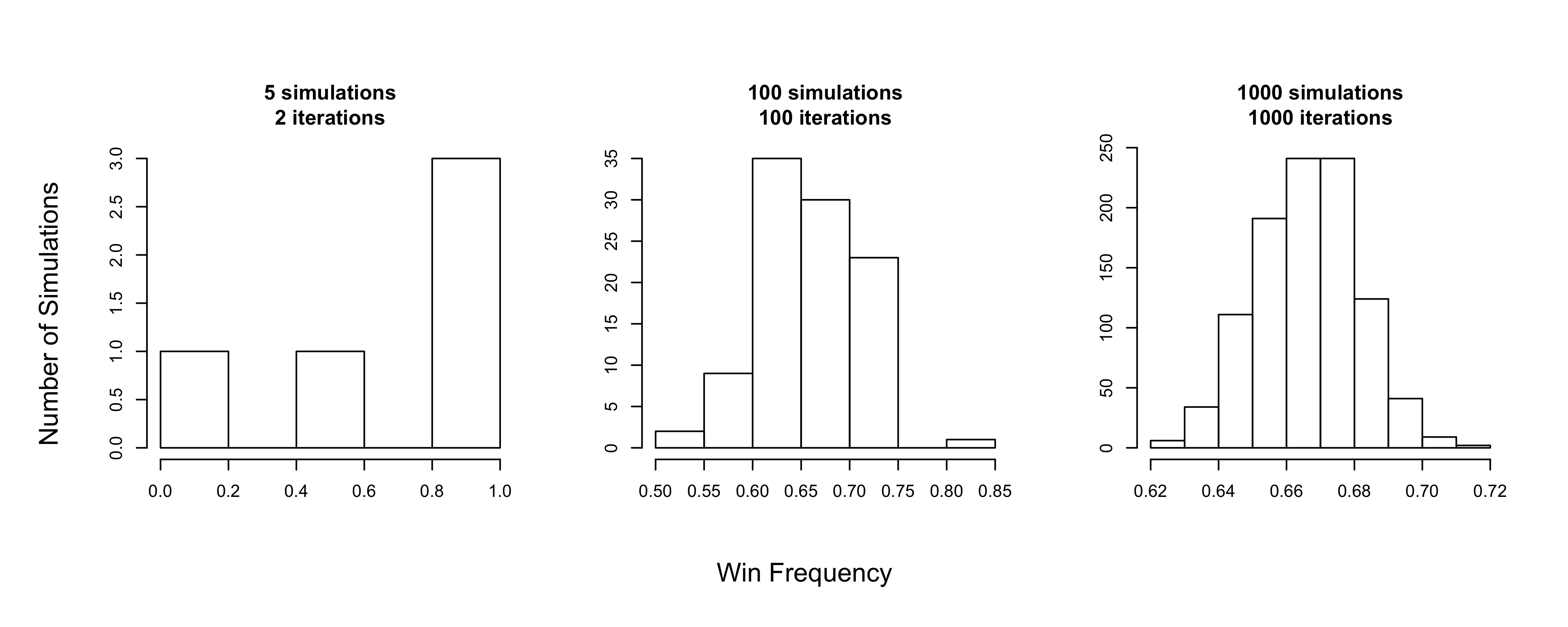
Figure 1. Composite histograms of Monty Hall simulation runs using classic parameters. At left is smallest run (5 simulations of 2 games, 10 games total), middle is intermediate run (100 simulations and games, 10,000 total games), right is largest run (1,000 simulations and games, 1,000,000 games total).
If you prefer to be more precise about the increase in distribution normality, we can apply the Shapiro-Wilk Normality test with shapiro.test() to test the null hypothesis that data were drawn from a normal distribution.
# run normality tests
    st1 <- shapiro.test(lr[["5;2"]])$p.value
    st2 <- shapiro.test(lr[["100;100"]])$p.value
    st3 <- shapiro.test(lr[["1000;1000"]])$p.value
With increased simulations and iterations, our p-value increased from 0.05 in the first and smallest run to 0.58 in the third and largest run. In other words, confidence decreases for rejecting the null hypothesis (normality) or accepting the alternative hypothesis (non-normality) as the underlying distributions converge to approximate normality.
Bending the game rules
I’ve written the simulation code to execute the Monty Hall problem with its classic characteristics by default, while allowing for modification of certain game rules and conditions. For our purposes, these classic parameters include randomization of the first 3 steps and that Monty reveals all but 1 door between player decisions. Changing other game conditions and studying the impact on win frequency distributions can help us better understand how the game ticks. In the process, visualizing our simulation results is a compelling way of reinforcing the notion that switching always increases win chances under the classic game rules.
The first condition I’ll explore is door quantity, which can be set with the ndoors argument to mhsim(). This value then gets passed to mhgame(). In practice this simply sets the doorseq vector of door indices to be of length ndoors, and subsequent steps proceed as normal.
Next, we can vary the player switch frequency (decision 2). The default setting doorswitch = 1 means the player switches 100% of the time, and this can be decreased to some decimal between 0 and 1. The player decision (switch or stay) is determined by randomly selecting from a weighted binomial distribution defined by the argument. So if doorswitch = 0.2, the player decision is drawn from a distribution where 20% of options are “switch” and (100 - 20 = ) 80% of options are “stay”. Again, setting this argument allows other game steps to run as normal.
Increasing door counts and visualizing the mnemonic device
Besides rote memorization, a useful mnemonic device to intuit or re-derive that we should always switch doors is to simply increase the number of doors while preserving the other default settings/game rules. Maybe we’re unsure if switching doors will increase our win chances with 3 doors. But if there’s instead 100 doors and Monty reveals goats behind 98 of them, it’s much clearer that switching will increase our chances of winning. As enumerated, we can quantitatively simulate outcome results from increasing the door quantity. Further, visualizing these results effectively can reinforce the intuition gained from this many-doors mnemonic device.
Let’s now generate and time the results of running 100 simulations of 100 classic games. I’ll vary ndoors from 3 to 103 by 10, with otherwise default settings (including that the player always switches their door choice).
# get win frequencies from varying ndoors
    simi = 100; iteri = 100
    ndoorl <- seq(3, 103, 10)
    seedl <- seq(1, 100, 1)
    lnd <- list()
    t1 <- Sys.time()
    for(nd in ndoorl){
      fw <- getfw(simi, iteri, nd)
      lnd[[paste0(nd)]] <- fw
    }
    tdif <- Sys.time() - t1
    # store the reference plot
    pref <- getlineplot(lnd, ptitle = "Canonical rules, varying doors")
All runs completed in about 5 seconds. Let’s visualize results in a few different ways. First, I’ll generate violin plots, a powerful way of showing density distributions. Because violin plots are relatively distribution-agnostic (e.g. no need to assume or imply distribution normality), they are often superior to traditional boxplots. Next, I’ll use overlapping density plots or “ridge plots.” These sometimes also called “joyplots” in homage to the iconic cover of Joy Division’s Unknown Pleasures record (awesome!). Finally, I’ll show line plots of run means with confidence boundaries. Where violin and ridge plots are relatively faithful representations of the underlying distributions, line plots use space a bit more efficiently and provide key characteristics of the plotted distributions.
To generate the plots, I’ve wrapped code into the utility functions getggdat() (format data for violin and ridge plots), getlinedat() (format data for line plots), getlineplot() (generate line plot object), getprettyplots() (generate composite of 3 ggplot2 plot types). I won’t explain these in depth here, but you may find these functions useful as a starting point towards a generalizable method to make these sorts of plots. This code makes use of some supremely awesome R packages that most data scientists will find useful, including ggplot2 (powerful plotting functions and meta syntax), gridExtra (managing plot outputs and composite plotting), and ggridges (ridge plot options).
png("mh_ndoors_3plots.png", width = 10, height = 4, units = "in", res = 400)
    getprettyplots(lnd, "Varying door count")
    dev.off()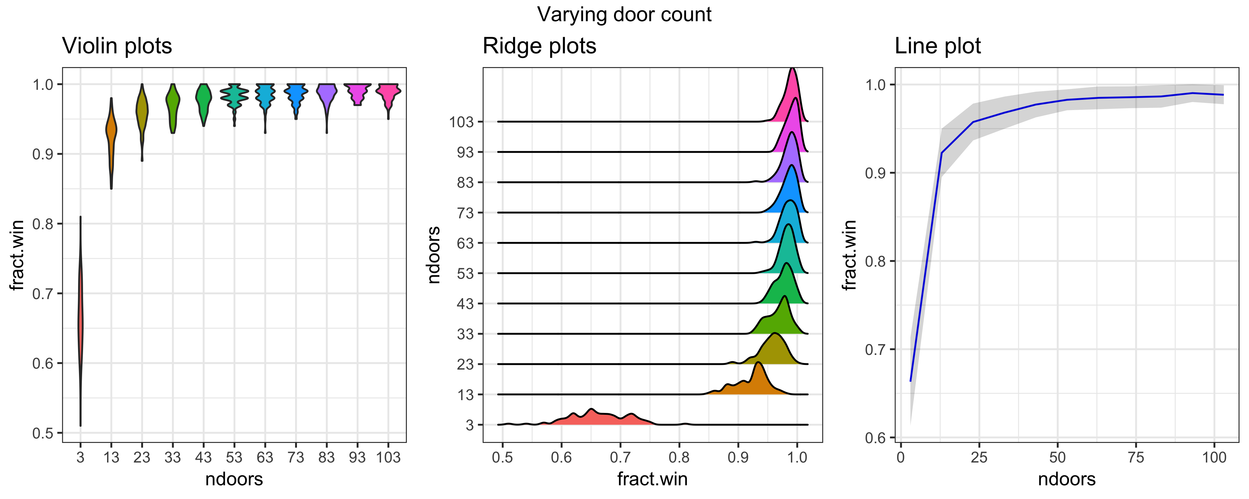
Figure 2. Three ways to visualize simulated win fraction distributions across door various quantities. Left, violin plots. Middle, ridge plots. Right, line plot of distribution means (lines) and standard deviation confidences (grey ribbon).
Thus we have 3 ways of visualizing the win frequency distribution increase following increased door quantity. Interestingly, as door quantity increases, the standard deviation seems to contract slightly after the means show an asymptote, which reflects that win frequency increase becomes both higher and more certain at higher door quantities.
I’ve allowed for two types of line plot overlays with the ribbontype argument. This allows for 2 types of confidence visualizations (the grey-colored ribbon overlay). Confidences can use either the standard deviation (if sd, the default), or the minimum and maximum win frequencies observed (if minmax). Let’s compare these below.
pclassic1 <- getlineplot(lnd, ptitle = "Std. dev. overlay", ribbontype = "sd")
    pclassic2 <- getlineplot(lnd, ptitle = "Min. max. overlay", ribbontype = "minmax")

    png("mh_2lineplots.png", width = 5, height = 3, units = "in", res = 400)
    grid.arrange(pclassic1, pclassic2, top = "Ribbon overlay comparison", ncol = 2)
    dev.off()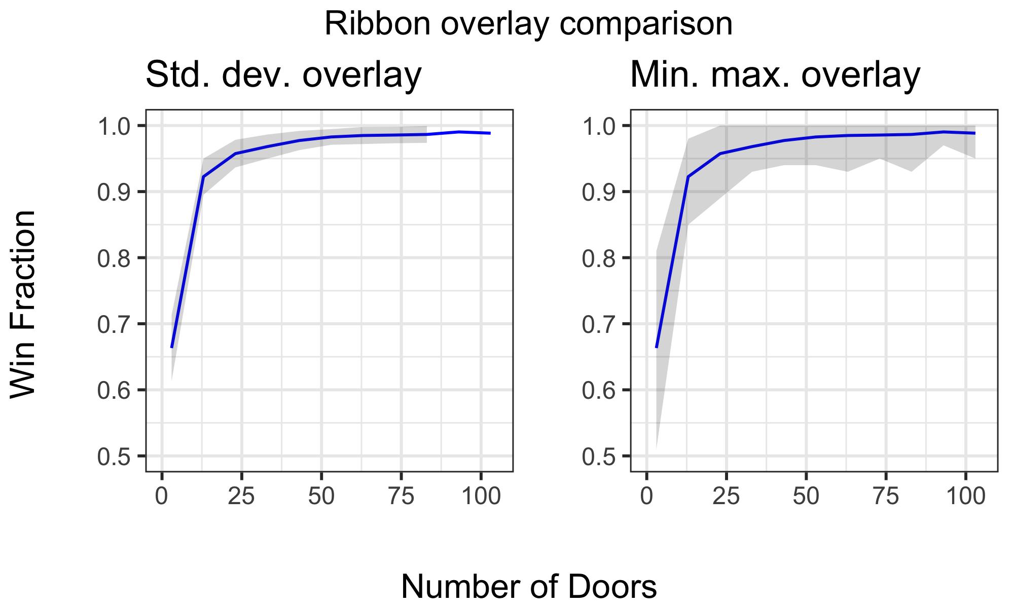
Figure 3. Line plot comparison showing 2 ways of visualizing win fraction distributions with door quantity. Left, grey confidence ribbon calculated using standard deviation. Right, confidences calculated from observed distribution minima and maxima.
Again, I’ll tend to use sd as it’s more useful to describe the underlying win fraction distributions being plotted.
What if the player doesn’t always switch?
Next, let’s observe the impact of changing the player switch frequency, or how often the player switches (player decision 2) from their initial door selection (decision 1). I’ll do this by varying the doorswitch argument, which parses player choice for each iteration from a weighted binomial distribution. I’ll also covary the door quantity with switch frequency, and observe outcome changes across both.
I’ll run 10 simulations varying the switch frequency from 0% to 100% in increments of 10%, and varying the door quantity as above (3 to 103 by 10). I’ll then store the results in ldat and the plots in plist. For the results plot, I’ve set identical x- and y-axis ranges in getlineplot to aid with visual comparison.
# get fwin dist across ndoors
    plist <- list()
    sfreq <- seq(0, 1, 0.1)
    t1 <- Sys.time()
    ldat <- list()
    for(s in sfreq){
      simi = 100; iteri = 100
      ndoorl <- seq(3, 103, 10)
      seedl <- seq(1, 100, 1)
      lnd <- list()
      for(nd in ndoorl){
        fw <- getfw(simi, iteri, nd, doorswitch = s)
        lnd[[paste0(nd)]] <- fw
      }
      plist[[paste0(s)]] <- getlineplot(lnd, ptitle = paste0("S.F. = ", s),
                                        xlim = c(0, 100), ylim = c(0, 1),
                                        xlab = "", ylab = "")
      ldat[[paste0(s)]] <- lnd
      # message(s)
    }
    tdif <- Sys.time() - t1
All runs completed in about 1 minute. The composite plot can now generated from plist.
png("mh_switchfreq.png", width = 10, height = 6, units = "in", res = 400)
    grid.arrange(plist[[1]], plist[[2]], plist[[3]],
                 plist[[4]], plist[[5]], plist[[6]],
                 plist[[7]], plist[[8]], plist[[9]],
                 plist[[10]],
                 ncol = 5,
                 bottom = "Number of Doors", left = "Win Fraction")
    dev.off()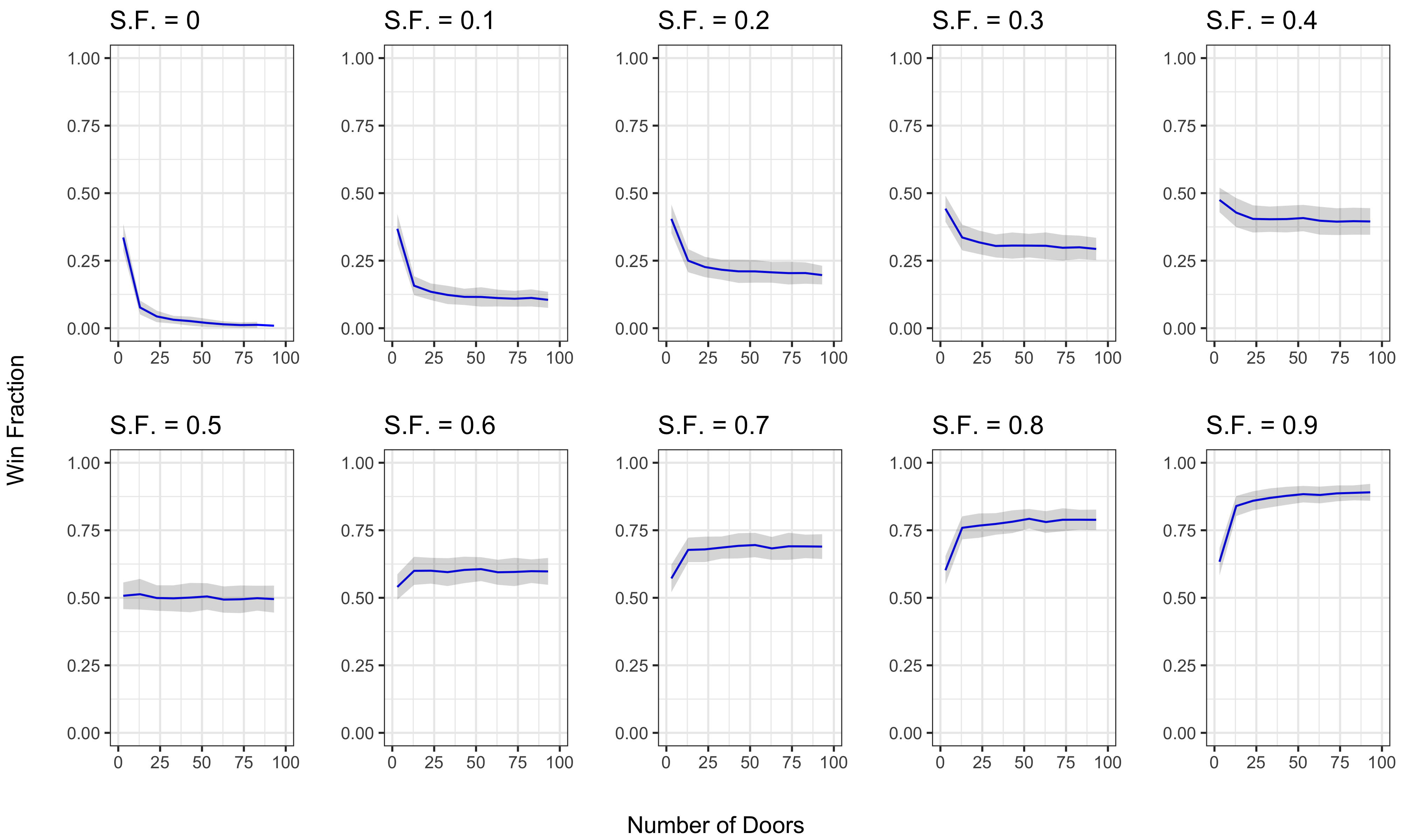
Figure 4. Composite line plots of ten simulation sets varying player switch frequency/fraction and door counts. Top row, first run to fifth run varying switch frequnecy from 0% to 40%. Bottom row, sixth run to final run varying switch frequency from 50% to 90%.
Across run sets of each door switch frequency, there’s a clear transition from an approximate negative power function (e.g. x ^ -1, top leftmost plot), to something approaching a fractional power function (e.g. x ^ 1/2, bottom rightmost plot). Note the win fraction only starts to show improvement with door quantity increase when the switch frequency is greater than 50% (bottom, second from leftmost plot), and that win fraction changes for a given switch frequency tend to always form asymptotes.
Increasing the switch frequency under classical rules should show progressive win fraction increases. Let’s generate and visualize the simulation results for this. I’ll appropriate my getlineplot() function, but note that it can be better to explicitly handle different axis variables (e.g. ndoors and doorswitch here) with discrete code.
sfreq <- seq(0, 1, 0.1)
    lnd <- list()
    for(s in sfreq){
      simi = 100; iteri = 100
      seedl <- seq(1, 100, 1)
      fw <- getfw(simi, iteri, doorswitch = s)
      lnd[[paste0(s)]] <- fw
    }
    png("mh_switchfreq_classicrules.png", width = 4, height = 4, res = 400, units = "in")
    getlineplot(lnd, ptitle = "Win Freq. by Switch Freq.",
                xlim = c(0, 1), ylim = c(0, 1),
                xlab = "Switch frequency")
    dev.off()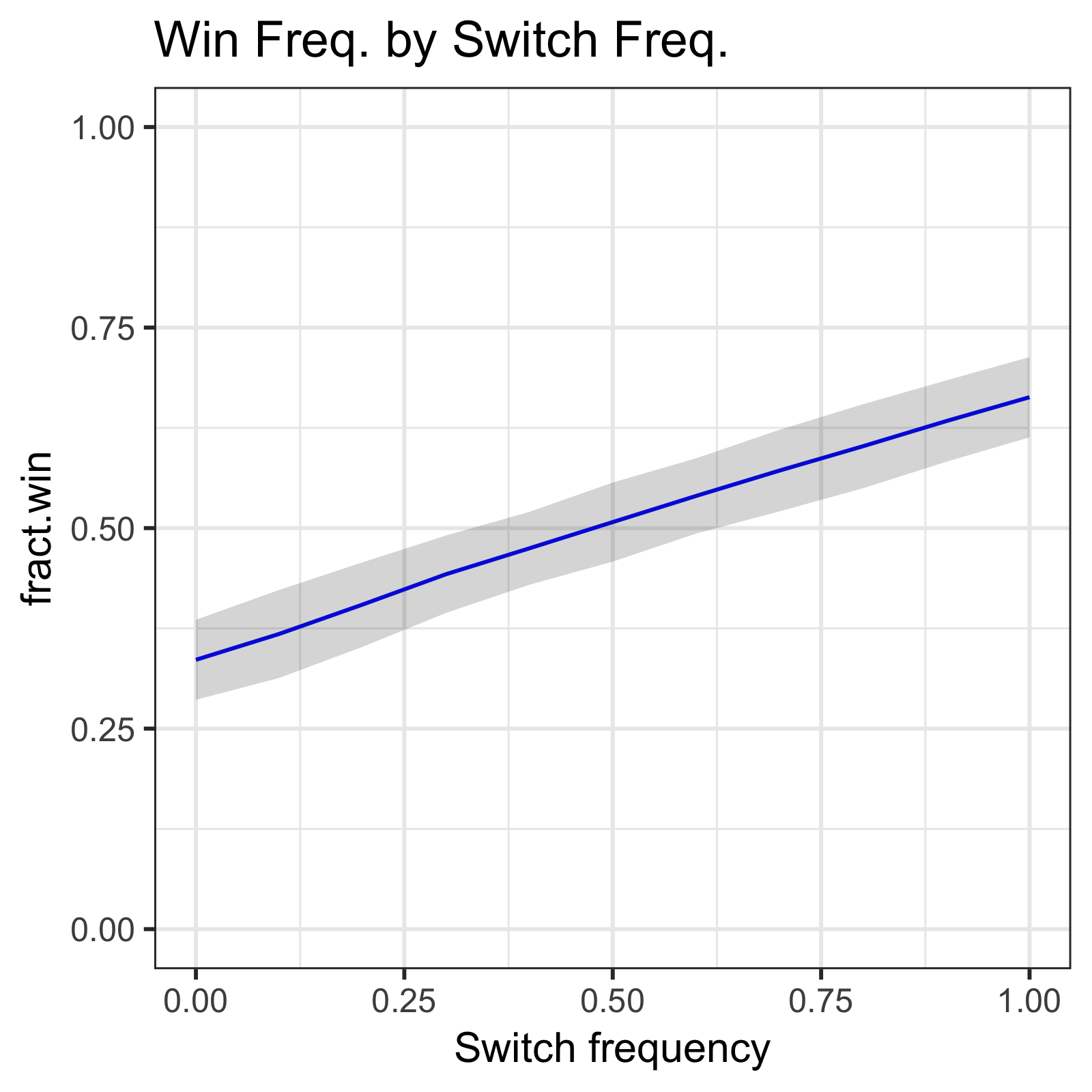
Figure 5. Simulation results from varying switch frequency using only classic Monty Hall rules/parameters (function defaults).
The resulting plot shows a clear linear win fraction increase with switch frequency, maxing out at the now-familiar mean of about 0.667.
Animating results plots
In data science, more tools in our toolkit means more options for tackling future problems. Here, I’ll illustrate how the ggplot2 meta syntax can be readily leveraged to generate useful plot animations. I’ve written the getprettygifs() function using the gganimate and magick packages and helpful code provided here to generate animated gifs of some of the plots above. I’ll generate these gifs using the results stored in the ldat list.
getprettygif(ldat[[11]], plottype = "composite_ndoors", gifname = "mh_ndoors.gif")
    getprettygif(ldat, plottype = "lineplots_doorswitch", gifname = "mh_switchfreq.gif")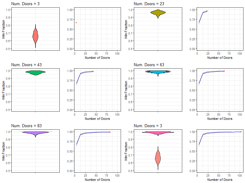
Figure 6. Animation of win fraction distributions from varying door quantity with otherwise classic rules. Left is violin plot animation, right is line plot animation. Title describes the nearest frame displayed.
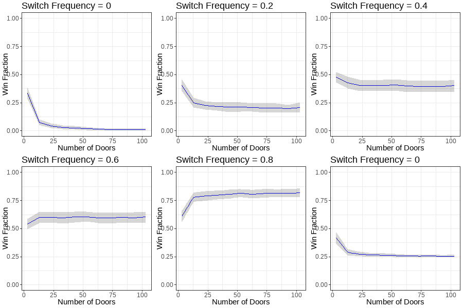
Figure 7. Animation of line plots showing win fraction distributions from varying player switch frequency and door quantities. Title describes the nearest frame displayed.
Conclusions and analysis extensions
I’ve explored simulations of the Monty Hall problem using a brute force approach. By exploring changes in win frequency across varying problem conditions, I’ve proven that switching doors will tend to increase player win frequency. I quantitatively investigated how always switching doors improves win frequency as door quantity increases, and visualized results to reinforce intuition from the many-doors mnemonic device. I also investigated how player switch frequency modifies win frequency gain or loss across door quantities. This showed recurrent asymptotic win frequency gain or loss, and how win frequency starts to improve with increase door quantity when the player switches over half the time.
This brute force simulation approach is one of many possible ways of sloving and exploring the Monty Hall problem. An alternate approach implementing Bayesian models could lead to further insights. There are several other game conditions that could also be explored, such as increasing the total number of doors with prizes. Ultimately, I hope this investigation provided some useful code and a framework for investigating new problems through simulation.
Further reading
Using R with NextFlow : Blog about using R and NextFlow to perform deconvolution algorithm benchmarks.
Run R package checks with a shell script : Blog about using a bash script to systematically run R package checks.